The Spambase data set consists of 4,601 e-mails, of which 1,813 are spam (39.4%). The data set archive contains a processed version of the e-mails wherein 57 real-valued features have been extracted and the spam/non-spam label has been assigned. You should work with this processed version of the data. The data set archive contains a description of the features extracted as well as some simple statistics over those features.
To estimate the generalization (testing) error of your classifier, you will perform cross-validation. In k-fold cross-validation, one would ordinarily partition the data set randomly into k groups of roughly equal size and perform k experiments (the "folds") wherein a model is trained on k-1 of the groups and tested on the remaining group, where each group is used for testing exactly once. (A common value of k is 10.) The generalization error of the classifier is estimated by the average of the performance across all k folds.
While one should perform cross-validation with random partitions, for consistency and comparability of your results, you should partition the data into 10 groups as follows: Consider the 4,601 data points in the order they appear in the processed data file. Each group will consist of every 10th data point in file order, i.e., Group 1 will consist of points {1,11,21,...}, Group 2 will consist of points {2,12,22,...}, ..., and Group 10 will consist of ponts {10,20,30,...}. Finally, Fold k will consist of testing on Group k a model obtained by training on the remaining k-1 groups.
The 57 features are real-valued, and one can model the feature distributions in simple and complex ways. You will explore the effect of this modeling on overall performance.
and use these estimated values in your Naive Bayes predictor, as appropriate. (I would suggest using Laplace or Laplace-like smoothing to avoid any issues with zero probabilities, and feel free to experiment with various theshold values, if you like.)
and estimate the class conditional probabilities for each of these bins, in a manner similar to that used in the Bernoulli model above. (Again, use Laplace smoothing to avoid any issues with zero probabilities, and feel free to experiment with the number of bins and various theshold values, if you like.)
When using Naive Bayes, one can easily make such trade-offs. For example, in the usual Bayes formulation, one would predict "spam" if
or equivalently, in a log-odds formulation,
Note that one could choose to classify an e-mail as spam for any threshold tau
where positive values of tau effectively reduce the number of spam classifications, thus decreasing false positives at the expense of increasing false negatives, while negative values of tau have the opposite effect.
One mechanism for visualizing this trade-off is through an ROC curve. (See, for example, the Wikipedia page on ROC curves.) An ROC curve effectively visualizes the true positive (detection) rate vs. the false positive (false alarm) rate for all possible thresholds. (The true positive rate is the fraction of spam messages above threshold; the false positive rate is the fraction of non-spam messages above threshold. Note that the true positive rate is 1 minus the false negative rate.)
One simple way to generate an ROC curve is to sort all m testing points by their log-odds, and for the top k testing points, for all k between 1 and m, calculate the true positive and false positive rates associated with the top k items; plot these points.
Create an ROC curve for each of your classifiers for Fold 1. Preferable draw all three curves on the same plot so that you can compare them.
The AUC can be calculated fairly simply using the trapezoidal rule for estimating the area under a curve: If our m ROC data points are
(x1, y1), (x2, y2), ..., (xm, ym)
in order, where
(x1, y1) = (0,0)
and
(xm, ym) = (1,1)
then the AUC is calculated as follows:
(1/2) sumk=2 to m (xk - xk-1) (yk + yk-1).
Calculate the AUC of your three classifiers.
a) Prove that
a) Somebody tosses a fair coin and if the result is heads, you
get nothing, otherwise you get $5. How much would you be pay to
play this game? What if the win is $500 instead of $5?
b) Suppose you play instead the following game: At the beginning of each game you pay an entry fee of $100. A coin is tossed until a head appears, counting n = the number of tosses it took to see the first head. Your reward is 2n (that is: if a head appears first at the 4th toss, you get $16). Would you be willing to play this game (why)?
c) Lets assume you answered "yes" at part b (if you did not, you
need to fix your math on expected values). What is the probability
that you make a profit in one game? How about in two games?
d) [difficult] After
about how many games (estimate) the probability of making a profit
overall is bigger than 50% ?
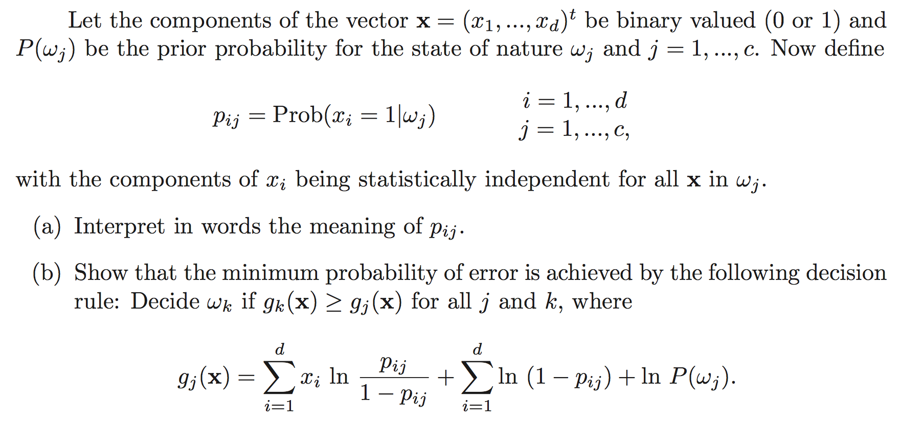
a) DHS CH2, Pb 45
