CS6220 Unsupervised Data Mining

HW3B tSNE, Feature Selection, Image HAAR Features

Make sure you check the syllabus for the due date. Please use the notations adopted in class, even if the problem is stated in the book using a different notation.

We are not looking for very long answers (if you find yourself writing more than one or two pages of typed text per problem, you are probably on the wrong track). Try to be concise; also keep in mind that good ideas and explanations matter more than exact details.

DATATSET : SpamBase: emails (54-feature vectors) classified as spam/nospam

DATATSET : 20 NewsGroups : news articles

DATATSET : MNIST : 28x28 digit B/W images

DATATSET : FASHION : 28x28 B/W images

https://en.wikipedia.org/wiki/MNIST_database
http://yann.lecun.com/exdb/mnist/
https://www.kaggle.com/zalando-research/fashionmnist

PROBLEM 1: tSNE dim reduction

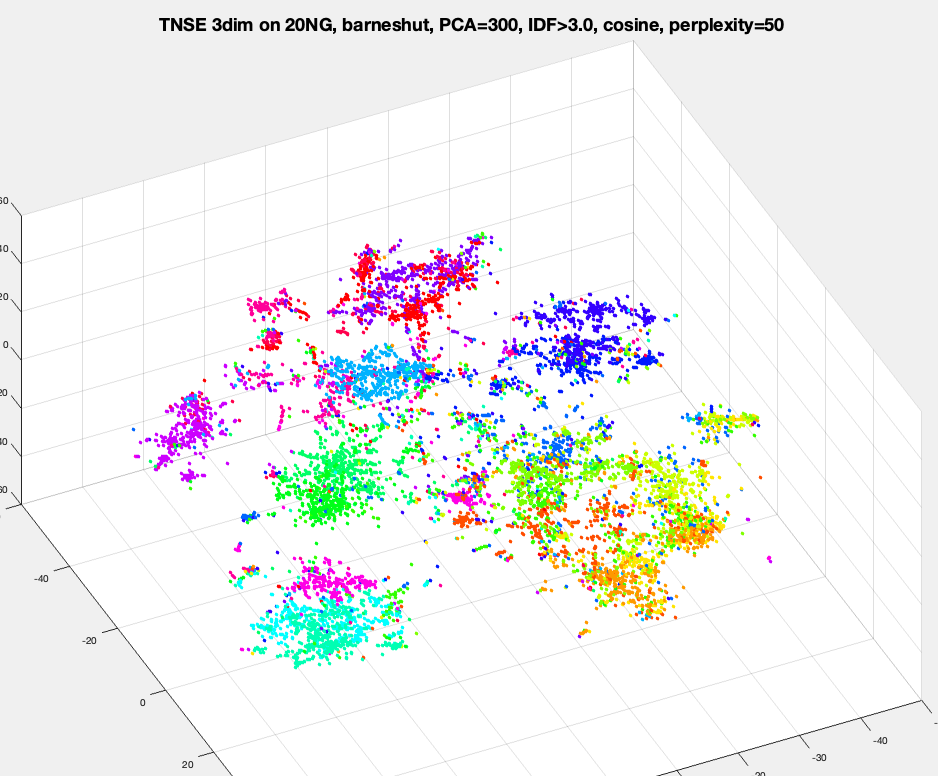
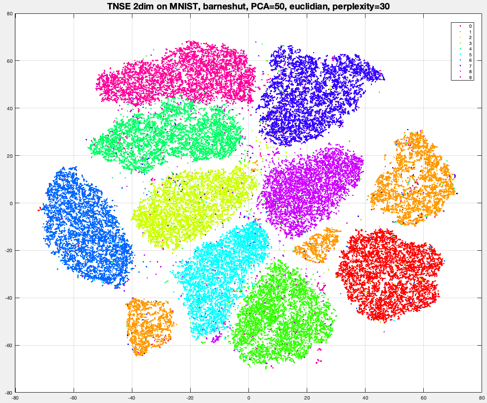
Run tSNE library/package on MNIST and 20NG datasets, to obtain a representation is 2-dim or 3-dim, and visualize the data by plotting datapoints with a color per label. Try different values for perplexity like 5, 20 and 100.

[Optional no credit] Run DBscan on tSNE-MNIST of G=2,3,5,10 dimensions. This should work much better than DBscan on original MNIST or on PCA-MNIST. You should be able to observe most datapoints "colored" and the colors roughly corresponding to image labels.

PROBLEM 2: Implement t-SNE dim reduction, run on MNIST dataset. The pseudocode/matlab below follows Laurens Van Der Maaten implementation

% load MNIST
W = load ('../../../data/mnist-original.mat');
X = W.data';
labels = W.label';
X = single(X);
% sample 10000 images
r = randperm(size(X,1));
ind = r(1:10000)';
X = X(ind, :);
labels = labels(ind);
%prep X
X = X - min(X(:)); %min_X=0
X = X / max(X(:)); %max _X=1
X = bsxfun(@minus, X, mean(X, 1));%0-mean

[N,F] = size(X);
no_dims=2;
PCA_dims =50;
use_momentum=1;

- run PCA
X = PCA(X, PCA_dims)

% compute pairwise distance
sum_X = sum(X .^ 2, 2);
D = bsxfun(@plus, sum_X, bsxfun(@plus, sum_X', -2 * (X * X')));

% compute the similarities p_ij for each row i:
P= zeros(N);
for i=1:N
beta=0.6;
D_i = D(i,:);
P_i = zeros(1,n);
% search for beta(i) so that i has effectively 30 neighbors: H =~ log2(30)
trials=0; Hdiff=1; betamin = -Inf; betamax = Inf;
while (abs(Hdiff)> 1e-5 and trials<50)
    P_i = exp(-D_i * beta);
    sumP = sum(P_i);
    H = log(sumP) + beta * sum(D_i .* P_i) / sumP;
    P_i = P_i / sumP;
    H_diff = H - log2(30);
    if (H_diff > 0)
       betamin = beta;
       if (betamax==+inf) beta = beta * 2;
       else beta = (beta + betamax) / 2;
       end
    end
    if (H_diff < 0)
       betamax = beta;
       if (betamin==-inf) beta = beta / 2;
       else beta = (beta + betamin) / 2;
       end
    end
trials=trials+1
end
beta(i) = beta;
P(i,:) = P_i; % write row i

end;
% make sure P is correct
P(i,i) = 0 for all i %0-diagonal
P = (P+P') /2 %symmetric
P = P ./ sum(P(:)) %normalized
ConstKL = sum(P(:) .* log(P(:)));

% initialize tSNE
max_iter = 400;
epsilon = 500;
min_gain = .01;
y = .0001 * randn(N, no_dims);
y_incs = zeros(size(y));
gains = ones(size(y));

% run tSNE iterations
for iter=1:max_iter
sum_y2 = sum(y .^ 2, 2);
% Student t-distribution as 1 / (1 + ||y_i - y_j||^2 )
Qnum = 1 ./ (1 + bsxfun(@plus, sum_y2, bsxfun(@plus, sum_y2', -2 * (y * y'))));
% fix Q
Q(i,i) = 0 for all i
Q = Qnum ./ sum(Qnum(:))

% compute y gradient matrix (each y_grads_i is 2-dim vector)
% y_grads_i = = 4*sum_j { (p_ij-q_ij) (y_i-y_j) / (1 + ||y_i - y_j||^2 ) }
% L_ij = = (p_ij-q_ij) / (1 + ||y_i - y_j||^2 ) }
L = (P - Q) .* Qnum;
% y_grads_i = = 4*sum_j { L_ij * (y_i-y_j) }
y_grads = 4 * (diag(sum(L, 1)) - L) * y;

if (use_momentum) % add momentum for grads in prev direction
    gains = (gains + .2) .* (sign(y_grads) ~= sign(y_incs)) + (gains * .8) .* (sign(y_grads) == sign(y_incs));
    gains(gains < min_gain) = min_gain;
    y_incs = - epsilon * (gains .* y_grads);
else %simple gradient descent
    y_incs = -epsilon * y_grads;
end;

% update y positions by gradients
y = y + y_incs;
y = bsxfun(@minus, y, mean(y, 1)); %recenter y with mean=0

% print loss and scatterplot every 10 iterations
if ~rem(iter, 10)
    cost = ConstKL - sum(P(:) .* log(Q(:)));
    disp(['Iteration ' num2str(iter) ': error is ' num2str(cost)]);
    figure(2); clf;
    scatter(y(:,1), y(:,2), 19, labels, 'filled');
    grid on; axis tight; axis on; drawnow
end
end

PROBLEM 3 : Pairwise Feature selection for text

On 20NG, run feature selection using skikit-learn built in "chi2" criteria to select top 200 features. Rerun a classification task, compare performance with HW3A-PB1. Then repeat the whole pipeline with "mutual-information" criteria.

PROBLEM 4 : L1 feature selection on text

Run a strongL1-regularized regression (library) on 20NG, and select 200 features (words) based on regression coefficients absolute value. Then reconstruct the dateaset with only these features, and rerun any of the classification tasks,

PROBLEM 5 HARR features for MNIST [Optional, no credit]

Implement and run HAAR feature Extraction for each image on the Digit Dataset. Then repeat the classification task with the extracted features.

HAAR features for Digits Dataset :First randomly select/generate 100 rectangles fitting inside 28x28 image box. A good idea (not mandatory) is to make rectangle be constrained to have approx 130-170 area, which implies each side should be at least 5. The set of rectangles is fixed for all images. For each image, extract two HAAR features per rectangle (total 200 features):

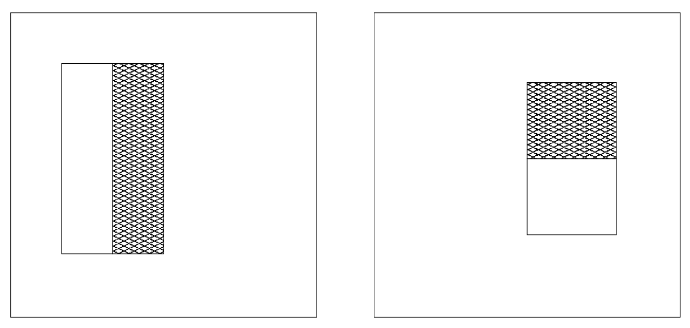
the black horizontal difference black(left-half) - black(right-half)
the black vertical difference black(top-half) - black(bottom-half)

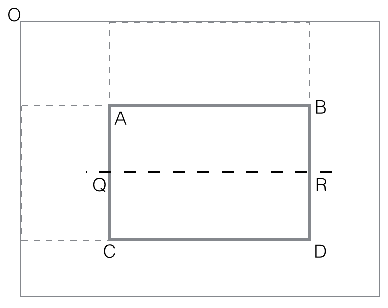
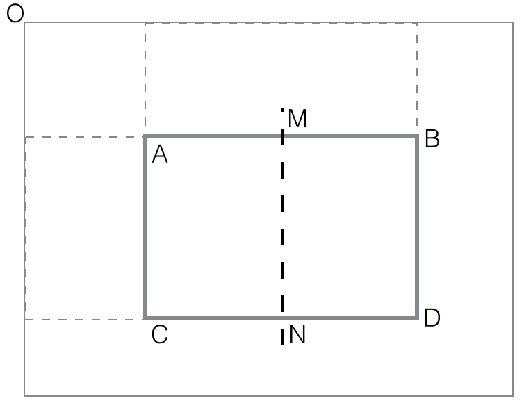
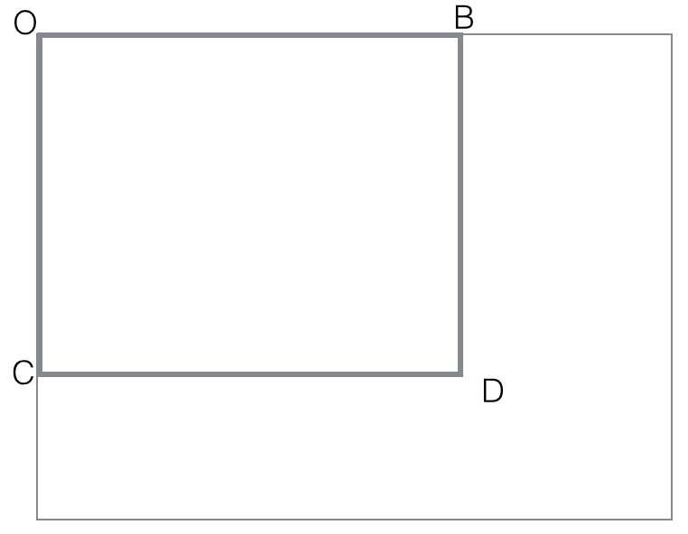
You will need to implement efficiently a method to compute the black amount (number of pixels) in a rectangle, essentially a procedure black(rectangle). Make sure you follow the idea presented in notes : first compute all black (rectangle OBCD) with O fixed corner of an image. These O-cornered rectangles can be computed efficiently with dynamic programming
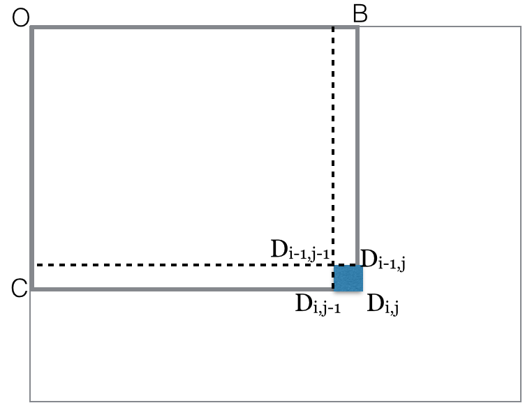
black(rectangle OBCD)= black(rectangle-diag(OD)) = count of black points in OBCD matrix
for i=rows
for j=columns
black(rectangle-diag(OD_ij)) = black(rectangle-diag(OD_i,j-1)) + black(rectangle-diag(OD_i-1,j))
- black(rectangle-diag(OD_i-1,j-1)) + black(pixel D_ij)
end for
end for

Assuming all such rectangles cornered at O have their black computed and stored, the procedure for general rectangles is quite easy:
black(rectangle ABCD) = black(OTYD) - black(OTXB) - black(OZYC) + black(OZXA)

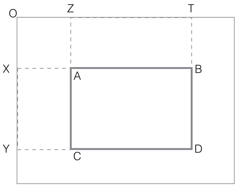
The last step is to compute the two feature (horizontal, vertical) values as differences:
vertical_feature_value(rectangle ABCD) = black(ABQR) - black(QRCD)
horizontal_feature_value(rectangle ABCD) = black(AMCN) - black(MBND)